Difference between revisions of "TrackingRobots"
| (5 intermediate revisions by the same user not shown) | |||
| Line 6: | Line 6: | ||
== OpenTLD description == | == OpenTLD description == | ||
| + | [[File:Tld.png|200px|thumb|left|TLD]] | ||
'''Overview''' | '''Overview''' | ||
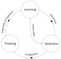
OpenTLD itself - as the name suggests - consists of three main parts: tracking learning and detection. Tracking estimates the object motion making an assumption that the object is visible in the beginning and fits all in the image from camera. Detector scans the full image and provides localization of all appearances of the object in the past. Learning take results from both, compares them, estimates errors and generates training examples to avoid those errors in the future. | OpenTLD itself - as the name suggests - consists of three main parts: tracking learning and detection. Tracking estimates the object motion making an assumption that the object is visible in the beginning and fits all in the image from camera. Detector scans the full image and provides localization of all appearances of the object in the past. Learning take results from both, compares them, estimates errors and generates training examples to avoid those errors in the future. | ||
'''Tracking''' | '''Tracking''' | ||
| − | Tracker uses optical flow estimation - mainly Lucas - Kanade method [ | + | [[File:Lk5.png|200px|thumb|right|Lucas-Kande - flow of the points]] |
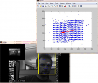
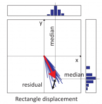
| + | Tracker uses optical flow estimation - mainly Lucas - Kanade method [3]. It accepts a pair of images and one bounding box as an input and outputs bounding box for the second image. For that it uses a set of points initialized on a regular grid (on the part of image isolated by the bounding box). Each of them have the LK method applied which generates a sparse motion flow between image 1 and image 2. Created in this way displacement is then recorded and histogram of all displacements is created. The error for each point is assigned based on the distance from the mean of this histogram (mean direction of the flow). 50% of the worst predictions are filtered out. All the other ones are moved in the direction of the mean and create a new bounding box. | ||
As a validator forward-backward error estimation is used. The whole above algorithm is run on consecutive frames creating a trajectory of bounding boxes. Then the same thing is run from the last frame to the first one. Error is estimated as a distance between bounding boxes on corresponding frames. | As a validator forward-backward error estimation is used. The whole above algorithm is run on consecutive frames creating a trajectory of bounding boxes. Then the same thing is run from the last frame to the first one. Error is estimated as a distance between bounding boxes on corresponding frames. | ||
| + | [[File:Tld1.png|200px|thumb|right|Median flow]] | ||
| + | [[File:Tld2.png|200px|thumb|right|Forward - Backward error estimation]] | ||
'''Detection''' | '''Detection''' | ||
| − | Detector uses the sliding window through the image of each frame and combines an offline trained face detector with online trained 1-NN (nearest neighbours) classifier. It tries to find patches (windows) on the image which represent objects similar to the tracked one. How close each of them is to the original (example given in the first bounding box) is measured by the distance(x_i,x_j)=1-NCC(x_i,x_j) where NCC is normalized cross-correlation. x_i represents a set of features which encodes the image i. This features are created using 2BitBP (2bit Binary Patterns) methods inspired by LBP (Local Binary Patterns) [ | + | Detector uses the sliding window through the image of each frame and combines an offline trained face detector with online trained 1-NN (nearest neighbours) classifier. It tries to find patches (windows) on the image which represent objects similar to the tracked one. How close each of them is to the original (example given in the first bounding box) is measured by the distance(x_i,x_j)=1-NCC(x_i,x_j) where NCC is normalized cross-correlation. x_i represents a set of features which encodes the image i. This features are created using 2BitBP (2bit Binary Patterns) methods inspired by LBP (Local Binary Patterns) [4] and similar to Haar-like features [5]. Each patch is encoded by many randomly chosen areas (randomly in a sense of position, scale and aspect ratio) which build them up. We split them into several groups. Each group of features represents then a different view of the object and is built into a tree which grows when the new positive feature examples come and prunned for negative ones. All of those trees build up together the sequential randomized forest. Single features are represented by one of the four possible codes which represent gradient descent in horizontal and vertical direction in the brightness of the image. |
Detection is made by putting each incoming patch from a sliding window through all of the trees in the forest. Each of them makes a decision whether an underlying patch is in the model or not. The decision is then made based on the majority vote. Each leaf records number of positive and negative examples and calculates posterior using maximal likelihood estimator P(y=1|x_i) = P/(P+N). Mean of it is then calculated and patches likely to represent an object are put into the classifier to measure their confidence through distance from the object example in the beginning. The rest of them is treated as background. | Detection is made by putting each incoming patch from a sliding window through all of the trees in the forest. Each of them makes a decision whether an underlying patch is in the model or not. The decision is then made based on the majority vote. Each leaf records number of positive and negative examples and calculates posterior using maximal likelihood estimator P(y=1|x_i) = P/(P+N). Mean of it is then calculated and patches likely to represent an object are put into the classifier to measure their confidence through distance from the object example in the beginning. The rest of them is treated as background. | ||
| + | |||
'''Learning''' | '''Learning''' | ||
Learning phase is conducted via P-N learning (Positive-Negative) which given a single patch and a video sequence, simultaneously learn an object classifier and label all patches in the video as ‘object’ (positive) or ‘background’ (negative). It uses a tracker for providing positive and detector for negative training examples. Both on them make errors and their compensation provides stability which produce new training examples. | Learning phase is conducted via P-N learning (Positive-Negative) which given a single patch and a video sequence, simultaneously learn an object classifier and label all patches in the video as ‘object’ (positive) or ‘background’ (negative). It uses a tracker for providing positive and detector for negative training examples. Both on them make errors and their compensation provides stability which produce new training examples. | ||
| Line 27: | Line 32: | ||
| − | + | [1] For controlling | |
http://www.usna.edu/Users/weapsys/esposito/roomba.matlab/ | http://www.usna.edu/Users/weapsys/esposito/roomba.matlab/ | ||
| − | + | [2] OpenTLD algorithm version used: | |
https://github.com/zk00006/OpenTLD | https://github.com/zk00006/OpenTLD | ||
| − | - | + | [3] http://en.wikipedia.org/wiki/Lucas%E2%80%93Kanade_method |
| + | |||
| + | [4] http://en.wikipedia.org/wiki/Local_binary_patterns | ||
| + | |||
| + | [5] http://en.wikipedia.org/wiki/Haar-like_features | ||
| + | |||
| + | [6] http://info.ee.surrey.ac.uk/Personal/Z.Kalal/ | ||
| + | |||
| + | [7] Z. Kalal, K. Mikolajczyk, and J. Matas, “Face-TLD: Tracking-Learning-Detection Applied to Faces,”International Conference on Image Processing, 2010. | ||
| + | |||
| + | [8] Z. Kalal, K. Mikolajczyk, and J. Matas, “Forward-Backward Error: Automatic Detection of Tracking Failures,” International Conference on Pattern Recognition, 2010, pp. 23-26. | ||
| + | |||
| + | [9] Z. Kalal, J. Matas, and K. Mikolajczyk, “P-N Learning: Bootstrapping Binary Classifiers by Structural Constraints,” Conference on Computer Vision and Pattern Recognition, 2010. | ||
| + | |||
| + | [10] Z. Kalal, J. Matas, and K. Mikolajczyk, “Online learning of robust object detectors during unstable tracking,” On-line Learning for Computer Vision Workshop, 2009. | ||
| + | |||
| + | [11] Z. Kalal, J. Matas, and K. Mikolajczyk, “Weighted Sampling for Large-Scale Boosting,” British Machine Vision Conference, 2008. | ||
| + | |||
| + | [12] NXT library http://www.mindstorms.rwth-aachen.de/trac/wiki/Download | ||
| + | |||
| + | [13] Base code: [[File:TLD_Roomba_NXT.zip]] | ||
| − | |||
| − | |||
| − | |||
| − | |||
| − | |||
| − | |||
| − | |||
| − | |||
| − | |||
| − | |||
| − | |||
| − | |||
== Support == | == Support == | ||
| Line 70: | Line 83: | ||
For linux openCV should be in the repositories. All you need to do is to compile GCC specific to MATLAB version. | For linux openCV should be in the repositories. All you need to do is to compile GCC specific to MATLAB version. | ||
| + | |||
| + | '''Installation''' | ||
| + | |||
| + | - Download files provided in references. | ||
| + | - Put everything into OpenTLD folder | ||
| + | - Compile and run algorithm | ||
Latest revision as of 04:12, 16 June 2011
Abstract
Connecting Roomba, NXT and OpenTLD algorithm together to build a robot which follows people or specific objects
OpenTLD description
Overview OpenTLD itself - as the name suggests - consists of three main parts: tracking learning and detection. Tracking estimates the object motion making an assumption that the object is visible in the beginning and fits all in the image from camera. Detector scans the full image and provides localization of all appearances of the object in the past. Learning take results from both, compares them, estimates errors and generates training examples to avoid those errors in the future.
Tracking
Tracker uses optical flow estimation - mainly Lucas - Kanade method [3]. It accepts a pair of images and one bounding box as an input and outputs bounding box for the second image. For that it uses a set of points initialized on a regular grid (on the part of image isolated by the bounding box). Each of them have the LK method applied which generates a sparse motion flow between image 1 and image 2. Created in this way displacement is then recorded and histogram of all displacements is created. The error for each point is assigned based on the distance from the mean of this histogram (mean direction of the flow). 50% of the worst predictions are filtered out. All the other ones are moved in the direction of the mean and create a new bounding box. As a validator forward-backward error estimation is used. The whole above algorithm is run on consecutive frames creating a trajectory of bounding boxes. Then the same thing is run from the last frame to the first one. Error is estimated as a distance between bounding boxes on corresponding frames.
Detection Detector uses the sliding window through the image of each frame and combines an offline trained face detector with online trained 1-NN (nearest neighbours) classifier. It tries to find patches (windows) on the image which represent objects similar to the tracked one. How close each of them is to the original (example given in the first bounding box) is measured by the distance(x_i,x_j)=1-NCC(x_i,x_j) where NCC is normalized cross-correlation. x_i represents a set of features which encodes the image i. This features are created using 2BitBP (2bit Binary Patterns) methods inspired by LBP (Local Binary Patterns) [4] and similar to Haar-like features [5]. Each patch is encoded by many randomly chosen areas (randomly in a sense of position, scale and aspect ratio) which build them up. We split them into several groups. Each group of features represents then a different view of the object and is built into a tree which grows when the new positive feature examples come and prunned for negative ones. All of those trees build up together the sequential randomized forest. Single features are represented by one of the four possible codes which represent gradient descent in horizontal and vertical direction in the brightness of the image. Detection is made by putting each incoming patch from a sliding window through all of the trees in the forest. Each of them makes a decision whether an underlying patch is in the model or not. The decision is then made based on the majority vote. Each leaf records number of positive and negative examples and calculates posterior using maximal likelihood estimator P(y=1|x_i) = P/(P+N). Mean of it is then calculated and patches likely to represent an object are put into the classifier to measure their confidence through distance from the object example in the beginning. The rest of them is treated as background.
Learning Learning phase is conducted via P-N learning (Positive-Negative) which given a single patch and a video sequence, simultaneously learn an object classifier and label all patches in the video as ‘object’ (positive) or ‘background’ (negative). It uses a tracker for providing positive and detector for negative training examples. Both on them make errors and their compensation provides stability which produce new training examples.
Modification
The idea is to control the robot for tracking humans or specified objects. The example code provides a base for further development with Roomba and NXT robots. Robot tracks the face and tries to adjust its pose to find the fastest way to the target. NXT with camera may be used for providing active vision.
References
[1] For controlling http://www.usna.edu/Users/weapsys/esposito/roomba.matlab/
[2] OpenTLD algorithm version used: https://github.com/zk00006/OpenTLD
[3] http://en.wikipedia.org/wiki/Lucas%E2%80%93Kanade_method
[4] http://en.wikipedia.org/wiki/Local_binary_patterns
[5] http://en.wikipedia.org/wiki/Haar-like_features
[6] http://info.ee.surrey.ac.uk/Personal/Z.Kalal/
[7] Z. Kalal, K. Mikolajczyk, and J. Matas, “Face-TLD: Tracking-Learning-Detection Applied to Faces,”International Conference on Image Processing, 2010.
[8] Z. Kalal, K. Mikolajczyk, and J. Matas, “Forward-Backward Error: Automatic Detection of Tracking Failures,” International Conference on Pattern Recognition, 2010, pp. 23-26.
[9] Z. Kalal, J. Matas, and K. Mikolajczyk, “P-N Learning: Bootstrapping Binary Classifiers by Structural Constraints,” Conference on Computer Vision and Pattern Recognition, 2010.
[10] Z. Kalal, J. Matas, and K. Mikolajczyk, “Online learning of robust object detectors during unstable tracking,” On-line Learning for Computer Vision Workshop, 2009.
[11] Z. Kalal, J. Matas, and K. Mikolajczyk, “Weighted Sampling for Large-Scale Boosting,” British Machine Vision Conference, 2008.
[12] NXT library http://www.mindstorms.rwth-aachen.de/trac/wiki/Download
[13] Base code: File:TLD Roomba NXT.zip
Support
Compiling OpenTLD For Windows 7 64:
- openCV
   - cmake (binaries for 32bits work well)
   - visual studio
   - windows sdk
   - create build folder (e.g. opencv/build64)
   - add source folder (e.g. opencv) and build folder to cmake
   - choose visual studio as compiler
   - click configure
   - click generate
   - go to build folder and open "opencv" file in visual studio
   - build and install everything (or parts you need)
   - add build path / bin to system PATH
   - change includes in compile.m file to fit your openCV installation
   - comment #ifdef _CHAR16T and following two lines in files lk.cpp, fern.cpp, bb_overlap.cpp (for MATLAB 2011; don't comment for 2010 version)
- matlab runtime compiler (other would receive "module could not be found" trying to load mex modules)
For linux openCV should be in the repositories. All you need to do is to compile GCC specific to MATLAB version.
Installation
   - Download files provided in references.
   - Put everything into OpenTLD folder
   - Compile and run algorithm


